── Attaching core tidyverse packages ──────────────────────── tidyverse 2.0.0 ──
✔ dplyr     1.1.3     ✔ readr     2.1.4
✔ forcats   1.0.0     ✔ stringr   1.5.0
✔ ggplot2   3.4.3     ✔ tibble    3.2.1
✔ lubridate 1.9.2     ✔ tidyr     1.3.0
✔ purrr     1.0.2
── Conflicts ────────────────────────────────────────── tidyverse_conflicts() ──
✖ dplyr::filter() masks stats::filter()
✖ dplyr::lag()    masks stats::lag()
ℹ Use the conflicted package (<http://conflicted.r-lib.org/>) to force all conflicts to become errors
── Attaching packages ────────────────────────────────────── tidymodels 1.1.1 ──

✔ broom        1.0.5     ✔ rsample      1.2.0
✔ dials        1.2.0     ✔ tune         1.1.2
✔ infer        1.0.4     ✔ workflows    1.1.3
✔ modeldata    1.2.0     ✔ workflowsets 1.0.1
✔ parsnip      1.1.1     ✔ yardstick    1.2.0
✔ recipes      1.0.8

── Conflicts ───────────────────────────────────────── tidymodels_conflicts() ──
✖ scales::discard() masks purrr::discard()
✖ dplyr::filter()   masks stats::filter()
✖ recipes::fixed()  masks stringr::fixed()
✖ dplyr::lag()      masks stats::lag()
✖ yardstick::spec() masks readr::spec()
✖ recipes::step()   masks stats::step()
• Search for functions across packages at https://www.tidymodels.org/find/Food Accesibility in the US
Josh, Stephany, Claire, Janie
Introduction and Data
Context
For our project, we are using a dataset about food access from the CORGIS Dataset Project. The data is originally from the United States Department of Agriculture’s Economic Research Service and comes from multiple sources. The population data, such as group quarter residences and population sizes of counties, were taken from the 2010 Census of the Population. Information on income-levels and access to vehicles came from American Community Survey responses from 2014-2018. The data for grocery stores is combined form two existing lists of grocery stores, and then divided into counties. Each observation is a county and its corresponding information on population, state, and how many people do or do not have stable access to food based on their distance from the nearest grocery store. Each observation also has data on how many children, seniors, people with low-income, and people without a car are far or close from food. The observations come from counties from all over the US.
Research Question
The focus of our project is such: What is the correlation between population density and food insecurity within US states (primarily within NC)?
Hypothesis
We hypothesize that individuals with lower income levels in areas of low population density are more likely to be in the “low access” pool; states with more people of lower-income and higher population densities are likely to have large portion of their population beyond a 10 mile distance from a nearest grocery store.
Purpose
When people live in food deserts, they don’t access convenient or stable access to healthy and fresh foods. The nearest grocery markets would be too far to make consistent trips, for example. We’d like to learn more about which populations are more likely to be affected by food deserts. The variables we foresee being relevant to our research would be the county (categorical), population size (quantitative), and the number of overall people, low-income individuals who are 1/2, 10, and 20 miles away from the nearest supermarket (quantitative variables). We’re particularly interested in North Carolina as this is where we attend school. It this case, it may be useful to view states (categorical) with differing Gross Domestic Products as an additional comparison to add nuance to our findings.
One potential ethical concern is whether the dataset includes underrepresented groups. Individuals in rural areas may be harder to find and survey. We need to take into account not only the percentage of the county population that lives geographically close enough to grocery stores, but also demographic factors like age that affect how they may or may not be able to get there, such as children and elderly individuals.
Literature Review
DOI: https://doi.org/10.1377/hlthaff.2015.0645
Summary: According to the research published by Craig Gunderson and James Ziliak, “food desert” is a term for a geographic area where residents have little to no access to groceries—particularly produce like fruits and vegetables. Generally, they are found in areas with small populations, and rural locations, and low income/educated residents. Towns with a high black population also tend to have less access to grocery stores. There are factors that officially identify an area as a food desert. Distance from the average home in the community to a grocery store, household resources (average income level, employment), and availability of community resources (public transportation, average income), are all defining characteristics. Approximately 6.2% of Americans—39.5 million people—lack access to nutritious foods. Food deserts exist for reasons such as transportation access, the existence of snack/convenience foods, income inequality, and business profits. Although the issue may seem difficult to tackle, there are potential solutions to this crisis. First, the government can incentivize grocery stores to open in underprivileged and rural areas. Similarly, growing the local agriculture industry can allow greater access to fresh produce. Cities can also implement programs to encourage healthier diets.
Analysis: This article directly supports the argument that factors such as population density and income level relate to levels of food accessibility. It claims that food deserts are most commonly found in rural areas with low household incomes—while also mentioning that the racial demographics of an area has a strong correlation to food access.
Bibliography:
Gunderson, Craig, and James P Ziliak. “Food Insecurity and Health Outcomes.” Health Affairs, Nov. 2015, www.healthaffairs.org/doi/10.1377/hlthaff.2015.0645.
Methodology
Data and Packages
High-Level Glance of Food Access Levels and Population Across the Country
| totalLowAccess | totalPop | state | proportion |
|---|---|---|---|
| 0 | 897934 | Delaware | 0.0000000 |
| 130 | 3574097 | Connecticut | 0.0000364 |
| 1051 | 1052567 | Rhode Island | 0.0009985 |
| 9094 | 8791894 | New Jersey | 0.0010344 |
| 5979 | 5773552 | Maryland | 0.0010356 |
| 8229 | 6547629 | Massachusetts | 0.0012568 |
| 70869 | 19378102 | New York | 0.0036572 |
| 57318 | 12702379 | Pennsylvania | 0.0045124 |
| 198184 | 37253956 | California | 0.0053198 |
| 66685 | 11536504 | Ohio | 0.0057803 |
| 127788 | 18801310 | Florida | 0.0067968 |
| 76623 | 9535483 | North Carolina | 0.0080356 |
| 80070 | 9883640 | Michigan | 0.0081013 |
| 10847 | 1316470 | New Hampshire | 0.0082395 |
| 11378 | 1360301 | Hawaii | 0.0083643 |
| 105355 | 9687653 | Georgia | 0.0108752 |
| 71400 | 6483802 | Indiana | 0.0110121 |
| 168918 | 12830632 | Illinois | 0.0131652 |
| 83840 | 6346105 | Tennessee | 0.0132113 |
| 89451 | 6724540 | Washington | 0.0133022 |
| 120484 | 8001024 | Virginia | 0.0150586 |
| 42291 | 2700551 | Nevada | 0.0156601 |
| 76492 | 4625364 | South Carolina | 0.0165375 |
| 47746 | 2763885 | Utah | 0.0172750 |
| 484675 | 25145561 | Texas | 0.0192748 |
| 77411 | 3831074 | Oregon | 0.0202061 |
| 12940 | 625741 | Vermont | 0.0206795 |
| 93183 | 4339367 | Kentucky | 0.0214739 |
| 110662 | 5029196 | Colorado | 0.0220039 |
| 29869 | 1328361 | Maine | 0.0224856 |
| 134388 | 5686986 | Wisconsin | 0.0236308 |
| 122530 | 4779736 | Alabama | 0.0256353 |
| 178347 | 5988927 | Missouri | 0.0297795 |
| 146763 | 4533372 | Louisiana | 0.0323739 |
| 70103 | 1852994 | West Virginia | 0.0378323 |
| 247526 | 6392017 | Arizona | 0.0387242 |
| 207745 | 5303925 | Minnesota | 0.0391682 |
| 74003 | 1567582 | Idaho | 0.0472084 |
| 193999 | 3751351 | Oklahoma | 0.0517144 |
| 157606 | 3046355 | Iowa | 0.0517359 |
| 157628 | 2853118 | Kansas | 0.0552476 |
| 171053 | 2915918 | Arkansas | 0.0586618 |
| 193028 | 2967297 | Mississippi | 0.0650518 |
| 126039 | 1826341 | Nebraska | 0.0690118 |
| 171987 | 2059179 | New Mexico | 0.0835221 |
| 51115 | 563626 | Wyoming | 0.0906896 |
| 64834 | 710231 | Alaska | 0.0912858 |
| 111252 | 989415 | Montana | 0.1124422 |
| 109940 | 814180 | South Dakota | 0.1350316 |
| 115849 | 672591 | North Dakota | 0.1722429 |
# A tibble: 3 × 4
totalLowAccess totalPop state proportion
<dbl> <int> <chr> <dbl>
1 111252 989415 Montana 0.112
2 115849 672591 North Dakota 0.172
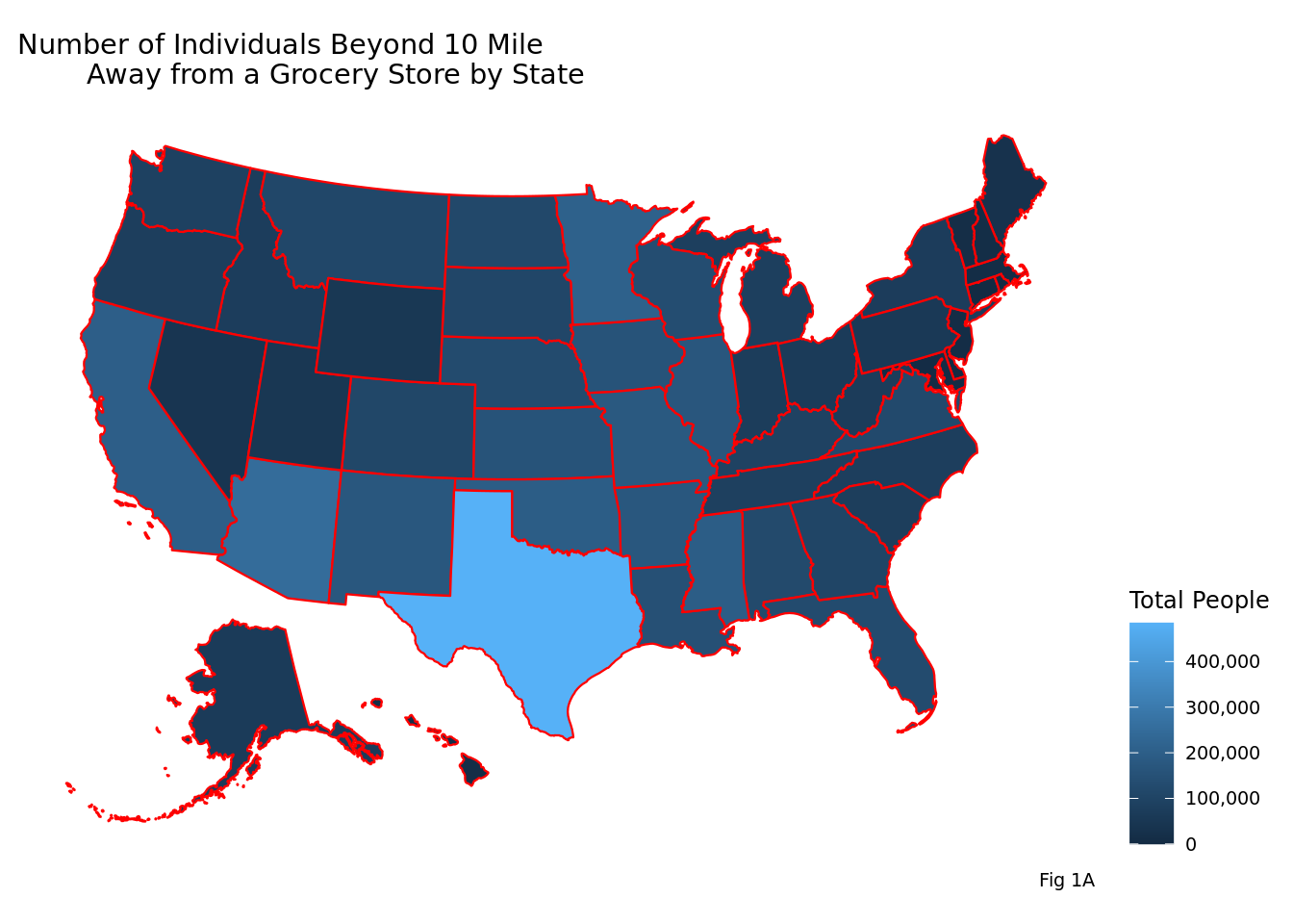
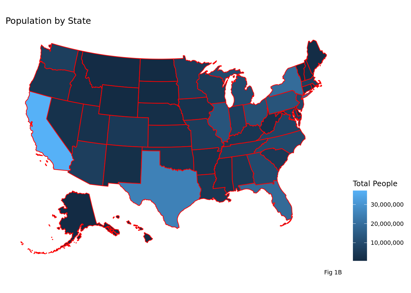
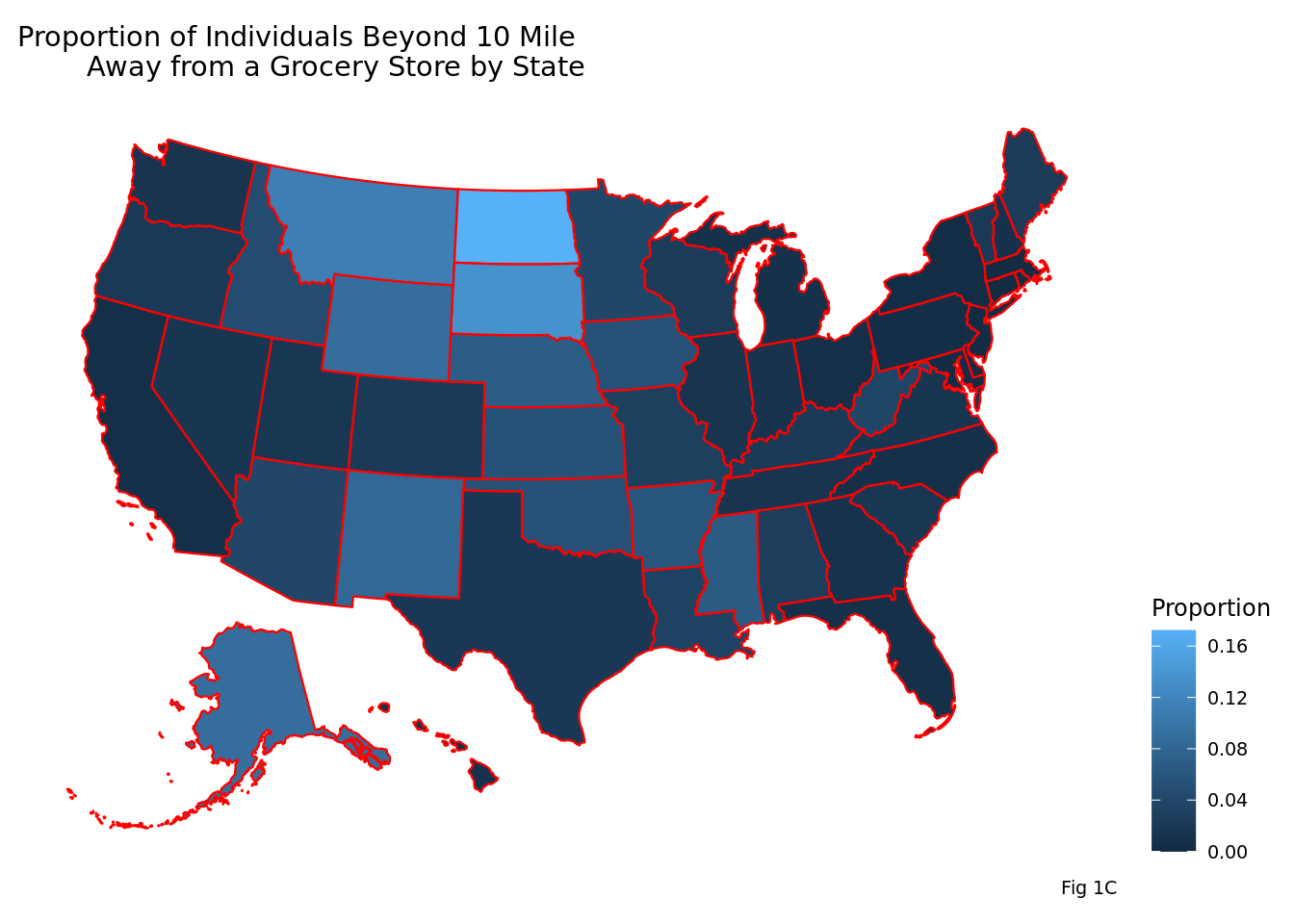
3 109940 814180 South Dakota 0.135Figure 1: These visualizations aid in understanding the relationship between individuals 10 miles from a grocery store by state and population. 10 miles was the unit chosen as it is a significant distance away from grocery stores. We will refer to these individuals as “low-access” due to this distance.
Comparing Food Access Levels Across Select States
| State | mean_low_access_1 | mean_low_access_1.2 | mean_low_access_10 | mean_low_access_20 | mean_population |
|---|---|---|---|---|---|
| Alabama | 43814.657 | 61155.925 | 1828.8060 | 3.477612 | 71339.34 |
| Alaska | 13218.276 | 19690.207 | 2235.6552 | 1399.517241 | 24490.72 |
| Arizona | 151312.867 | 302926.733 | 16501.7333 | 5843.400000 | 426134.47 |
| Arkansas | 23659.040 | 33280.227 | 2280.7067 | 27.906667 | 38878.91 |
| California | 118662.276 | 327716.241 | 3416.9655 | 581.517241 | 642309.59 |
| Colorado | 27049.562 | 56624.562 | 1729.0938 | 362.406250 | 78581.19 |
| Connecticut | 187277.625 | 329591.375 | 16.2500 | 0.000000 | 446762.12 |
| Delaware | 136739.000 | 227654.000 | 0.0000 | 0.000000 | 299311.33 |
| District of Columbia | 27650.000 | 196290.000 | 0.0000 | 0.000000 | 601723.00 |
| Florida | 98088.313 | 196422.030 | 1907.2836 | 62.194030 | 280616.57 |
| Georgia | 33372.447 | 50328.874 | 662.6101 | 2.842767 | 60928.64 |
| Hawaii | 101113.400 | 172927.400 | 2275.6000 | 50.800000 | 272060.20 |
| Idaho | 17272.341 | 27773.841 | 1681.8864 | 446.590909 | 35626.86 |
| Illinois | 39451.990 | 78892.402 | 1656.0588 | 0.000000 | 125790.51 |
| Indiana | 38614.120 | 58005.065 | 776.0870 | 0.000000 | 70476.11 |
| Iowa | 14088.515 | 23173.081 | 1591.9798 | 0.000000 | 30771.26 |
| Kansas | 11886.581 | 20861.933 | 1501.2190 | 42.542857 | 27172.55 |
| Kentucky | 21099.150 | 30116.100 | 776.5250 | 0.000000 | 36161.39 |
| Louisiana | 35434.094 | 55207.781 | 2293.1719 | 44.468750 | 70833.94 |
| Maine | 54064.812 | 68471.812 | 1866.8125 | 161.000000 | 83022.56 |
| Maryland | 85222.750 | 166981.667 | 249.1250 | 0.000000 | 240564.67 |
| Massachusetts | 168018.286 | 310229.571 | 587.7857 | 0.000000 | 467687.79 |
| Michigan | 55255.530 | 91853.542 | 964.6988 | 65.626506 | 119080.00 |
| Minnesota | 29218.943 | 46969.885 | 2387.8736 | 96.356322 | 60964.66 |
| Mississippi | 24853.207 | 32063.402 | 2354.0000 | 2.036585 | 36186.55 |
| Missouri | 25320.226 | 40905.122 | 1550.8435 | 19.330435 | 52077.63 |
| Montana | 9119.286 | 13369.071 | 1986.6429 | 811.017857 | 17668.12 |
| Nebraska | 7330.344 | 14166.011 | 1355.2581 | 122.096774 | 19638.08 |
| Nevada | 44049.765 | 100140.647 | 2487.7059 | 1014.058824 | 158855.94 |
| New Hampshire | 85858.100 | 111707.300 | 1084.7000 | 9.100000 | 131647.00 |
| New Jersey | 125782.524 | 250974.095 | 433.0476 | 0.000000 | 418661.62 |
| New Mexico | 30703.394 | 48395.909 | 5211.7273 | 2193.939394 | 62399.36 |
| New York | 73224.145 | 132327.242 | 1143.0484 | 5.951613 | 312550.03 |
| North Carolina | 53303.880 | 78983.900 | 766.2300 | 12.910000 | 95354.83 |
| North Dakota | 5575.170 | 9381.962 | 2185.8302 | 527.037736 | 12690.40 |
| Ohio | 60490.443 | 101384.216 | 757.7841 | 0.000000 | 131096.64 |
| Oklahoma | 24791.857 | 38550.455 | 2519.4675 | 77.064935 | 48718.84 |
| Oregon | 35885.667 | 70521.083 | 2150.3056 | 519.916667 | 106418.72 |
| Pennsylvania | 80890.328 | 134228.925 | 855.4925 | 0.000000 | 189587.75 |
| Rhode Island | 68650.600 | 145445.000 | 210.2000 | 0.000000 | 210513.40 |
| South Carolina | 61244.739 | 86164.609 | 1662.8696 | 16.086956 | 100551.39 |
| South Dakota | 6522.227 | 9763.348 | 1665.7576 | 255.939394 | 12336.06 |
| Tennessee | 39474.126 | 56498.011 | 882.5263 | 0.000000 | 66801.11 |
| Texas | 39244.016 | 73109.669 | 1908.1693 | 152.019685 | 98998.27 |
| Utah | 30739.345 | 68147.138 | 1646.4138 | 665.068965 | 95306.38 |
| Vermont | 28754.857 | 36888.429 | 924.2857 | 0.000000 | 44695.79 |
| Virginia | 25673.842 | 44370.925 | 905.8947 | 4.413534 | 60158.08 |
| Washington | 66519.897 | 121181.538 | 2293.6154 | 186.538462 | 172424.10 |
| West Virginia | 22336.418 | 28747.364 | 1274.6000 | 10.327273 | 33690.80 |
| Wisconsin | 37313.361 | 60407.278 | 1866.5000 | 16.527778 | 78985.92 |
| Wyoming | 13872.087 | 20284.348 | 2222.3913 | 787.086957 | 24505.48 |
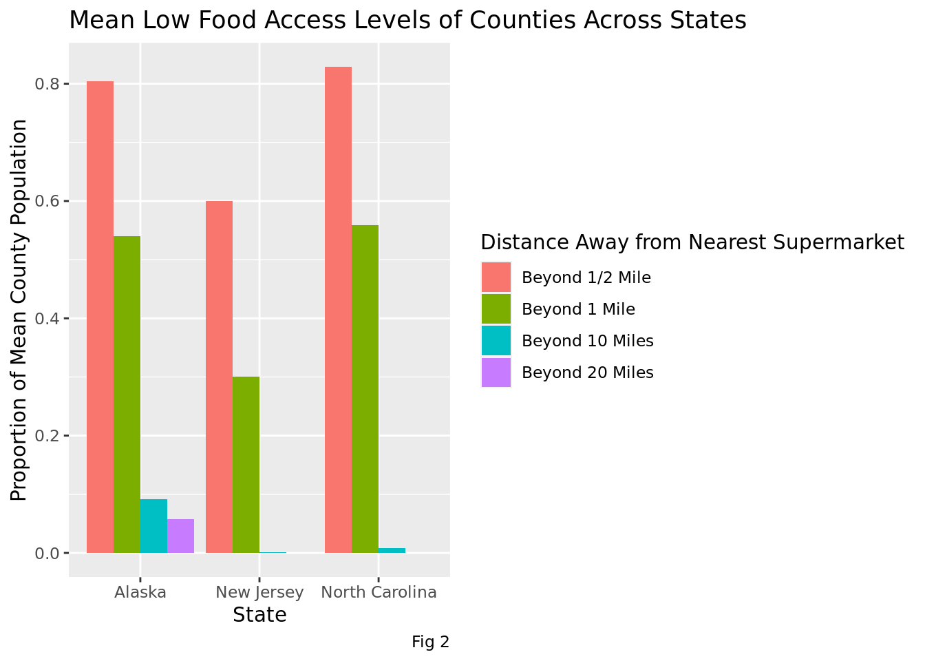
Figure 2: From the graph, we can see that on average, 5% (proportion of 0.05) of Alaska counties’ populations reside over 20 miles away and 9% (proportion of 0.09) reside over 10 miles away from a nearest grocery store, both of which are considerably larger proportions than for New Jersey and North Carolina counties.
Warning: Transformation introduced infinite values in continuous y-axis
Transformation introduced infinite values in continuous y-axis
Warning: Removed 32 rows containing non-finite values (`stat_ydensity()`).Warning: Removed 32 rows containing non-finite values (`stat_boxplot()`).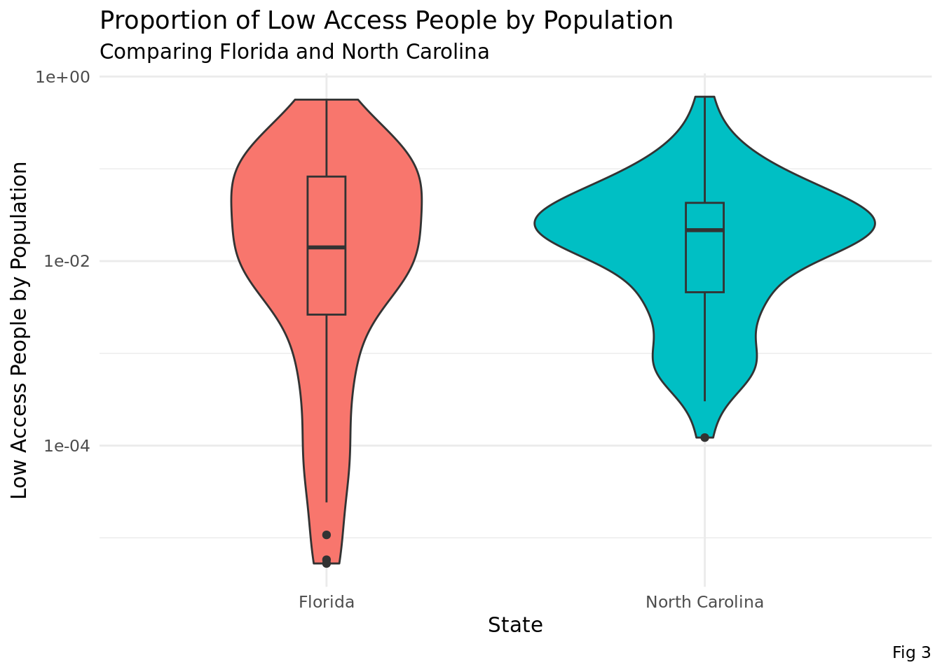
Figure 3: This figure aids in understanding the proportion of low access people within 10 miles of a supermarket by population in Florida and North Carolina. Florida was chosen as the proportions, median and mean, were approximately the same as North Carolina’s. When breaking it down by states, the plot shows the frequencies in the distribution of low-access individuals relative to population density with a boxplot to indicate the median, quartiles, and outliers in the data.
How Does Food Access Relate to Population Density in States?
Joining with `by = join_by(state)`| state | Resident.Population.Density | totalLowAccess | totalPop | proportion |
|---|---|---|---|---|
| Alabama | 94.4 | 122530 | 4779736 | 0.0256353 |
| Alaska | 1.2 | 64834 | 710231 | 0.0912858 |
| Arizona | 56.3 | 247526 | 6392017 | 0.0387242 |
| Arkansas | 56 | 171053 | 2915918 | 0.0586618 |
| California | 239.1 | 198184 | 37253956 | 0.0053198 |
| Colorado | 48.5 | 110662 | 5029196 | 0.0220039 |
| Connecticut | 738.1 | 130 | 3574097 | 0.0000364 |
| Delaware | 460.8 | 0 | 897934 | 0.0000000 |
| Florida | 350.6 | 127788 | 18801310 | 0.0067968 |
| Georgia | 168.4 | 105355 | 9687653 | 0.0108752 |
| Hawaii | 211.8 | 11378 | 1360301 | 0.0083643 |
| Idaho | 19 | 74003 | 1567582 | 0.0472084 |
| Illinois | 231.1 | 168918 | 12830632 | 0.0131652 |
| Indiana | 181 | 71400 | 6483802 | 0.0110121 |
| Iowa | 54.5 | 157606 | 3046355 | 0.0517359 |
| Kansas | 34.9 | 157628 | 2853118 | 0.0552476 |
| Kentucky | 109.9 | 93183 | 4339367 | 0.0214739 |
| Louisiana | 104.9 | 146763 | 4533372 | 0.0323739 |
| Maine | 43.1 | 29869 | 1328361 | 0.0224856 |
| Maryland | 594.8 | 5979 | 5773552 | 0.0010356 |
| Massachusetts | 839.4 | 8229 | 6547629 | 0.0012568 |
| Michigan | 174.8 | 80070 | 9883640 | 0.0081013 |
| Minnesota | 66.6 | 207745 | 5303925 | 0.0391682 |
| Mississippi | 63.2 | 193028 | 2967297 | 0.0650518 |
| Missouri | 87.1 | 178347 | 5988927 | 0.0297795 |
| Montana | 6.8 | 111252 | 989415 | 0.1124422 |
| Nebraska | 23.8 | 126039 | 1826341 | 0.0690118 |
| Nevada | 24.6 | 42291 | 2700551 | 0.0156601 |
| New Hampshire | 147 | 10847 | 1316470 | 0.0082395 |
| New Jersey | 1,195.50 | 9094 | 8791894 | 0.0010344 |
| New Mexico | 17 | 171987 | 2059179 | 0.0835221 |
| New York | 411.2 | 70869 | 19378102 | 0.0036572 |
| North Carolina | 196.1 | 76623 | 9535483 | 0.0080356 |
| North Dakota | 9.7 | 115849 | 672591 | 0.1722429 |
| Ohio | 282.3 | 66685 | 11536504 | 0.0057803 |
| Oklahoma | 54.7 | 193999 | 3751351 | 0.0517144 |
| Oregon | 39.9 | 77411 | 3831074 | 0.0202061 |
| Pennsylvania | 283.9 | 57318 | 12702379 | 0.0045124 |
| Rhode Island | 1,018.10 | 1051 | 1052567 | 0.0009985 |
| South Carolina | 153.9 | 76492 | 4625364 | 0.0165375 |
| South Dakota | 10.7 | 109940 | 814180 | 0.1350316 |
| Tennessee | 153.9 | 83840 | 6346105 | 0.0132113 |
| Texas | 96.3 | 484675 | 25145561 | 0.0192748 |
| Utah | 33.6 | 47746 | 2763885 | 0.0172750 |
| Vermont | 67.9 | 12940 | 625741 | 0.0206795 |
| Virginia | 202.6 | 120484 | 8001024 | 0.0150586 |
| Washington | 101.2 | 89451 | 6724540 | 0.0133022 |
| West Virginia | 77.1 | 70103 | 1852994 | 0.0378323 |
| Wisconsin | 105 | 134388 | 5686986 | 0.0236308 |
| Wyoming | 5.8 | 51115 | 563626 | 0.0906896 |
Joining with `by = join_by(state)`
`geom_smooth()` using formula = 'y ~ x'
Warning: Removed 1 rows containing missing values (`geom_text()`).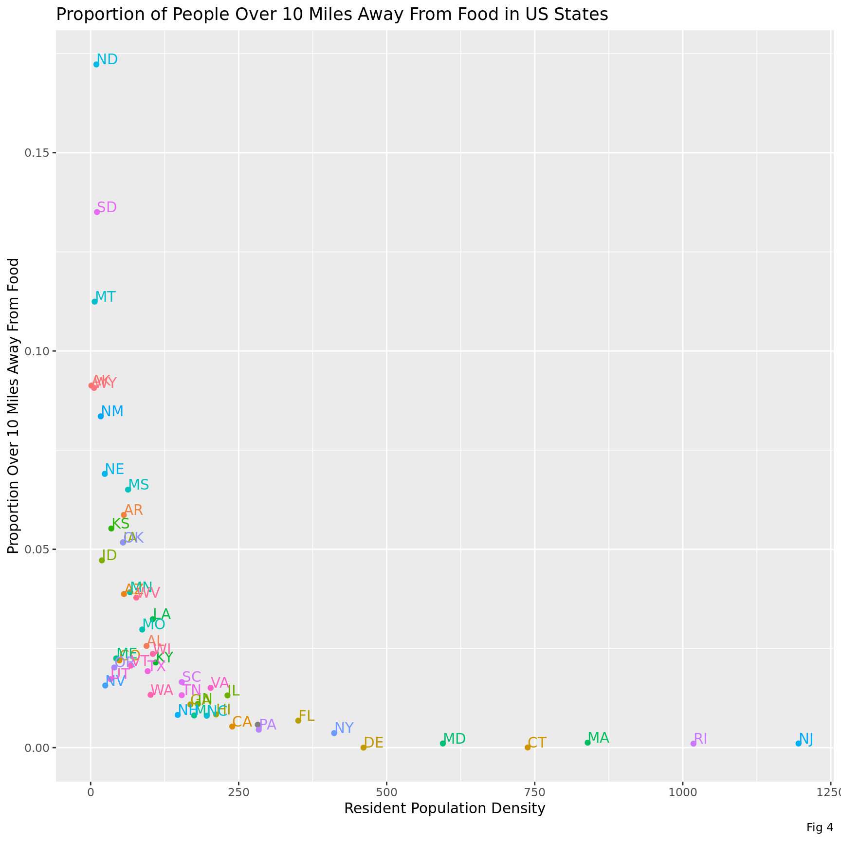
| state | Resident.Population.Density | totalLowAccess | totalPop | proportion | rpdens |
|---|---|---|---|---|---|
| Alabama | 94.4 | 122530 | 4779736 | 0.0256353 | 94.4 |
| Alaska | 1.2 | 64834 | 710231 | 0.0912858 | 1.2 |
| Arizona | 56.3 | 247526 | 6392017 | 0.0387242 | 56.3 |
| Arkansas | 56 | 171053 | 2915918 | 0.0586618 | 56.0 |
| California | 239.1 | 198184 | 37253956 | 0.0053198 | 239.1 |
| Colorado | 48.5 | 110662 | 5029196 | 0.0220039 | 48.5 |
| Connecticut | 738.1 | 130 | 3574097 | 0.0000364 | 738.1 |
| Delaware | 460.8 | 0 | 897934 | 0.0000000 | 460.8 |
| Florida | 350.6 | 127788 | 18801310 | 0.0067968 | 350.6 |
| Georgia | 168.4 | 105355 | 9687653 | 0.0108752 | 168.4 |
| Hawaii | 211.8 | 11378 | 1360301 | 0.0083643 | 211.8 |
| Idaho | 19 | 74003 | 1567582 | 0.0472084 | 19.0 |
| Illinois | 231.1 | 168918 | 12830632 | 0.0131652 | 231.1 |
| Indiana | 181 | 71400 | 6483802 | 0.0110121 | 181.0 |
| Iowa | 54.5 | 157606 | 3046355 | 0.0517359 | 54.5 |
| Kansas | 34.9 | 157628 | 2853118 | 0.0552476 | 34.9 |
| Kentucky | 109.9 | 93183 | 4339367 | 0.0214739 | 109.9 |
| Louisiana | 104.9 | 146763 | 4533372 | 0.0323739 | 104.9 |
| Maine | 43.1 | 29869 | 1328361 | 0.0224856 | 43.1 |
| Maryland | 594.8 | 5979 | 5773552 | 0.0010356 | 594.8 |
| Massachusetts | 839.4 | 8229 | 6547629 | 0.0012568 | 839.4 |
| Michigan | 174.8 | 80070 | 9883640 | 0.0081013 | 174.8 |
| Minnesota | 66.6 | 207745 | 5303925 | 0.0391682 | 66.6 |
| Mississippi | 63.2 | 193028 | 2967297 | 0.0650518 | 63.2 |
| Missouri | 87.1 | 178347 | 5988927 | 0.0297795 | 87.1 |
| Montana | 6.8 | 111252 | 989415 | 0.1124422 | 6.8 |
| Nebraska | 23.8 | 126039 | 1826341 | 0.0690118 | 23.8 |
| Nevada | 24.6 | 42291 | 2700551 | 0.0156601 | 24.6 |
| New Hampshire | 147 | 10847 | 1316470 | 0.0082395 | 147.0 |
| New Jersey | 1,195.50 | 9094 | 8791894 | 0.0010344 | 1195.5 |
| New Mexico | 17 | 171987 | 2059179 | 0.0835221 | 17.0 |
| New York | 411.2 | 70869 | 19378102 | 0.0036572 | 411.2 |
| North Carolina | 196.1 | 76623 | 9535483 | 0.0080356 | 196.1 |
| North Dakota | 9.7 | 115849 | 672591 | 0.1722429 | 9.7 |
| Ohio | 282.3 | 66685 | 11536504 | 0.0057803 | 282.3 |
| Oklahoma | 54.7 | 193999 | 3751351 | 0.0517144 | 54.7 |
| Oregon | 39.9 | 77411 | 3831074 | 0.0202061 | 39.9 |
| Pennsylvania | 283.9 | 57318 | 12702379 | 0.0045124 | 283.9 |
| Rhode Island | 1,018.10 | 1051 | 1052567 | 0.0009985 | 1018.1 |
| South Carolina | 153.9 | 76492 | 4625364 | 0.0165375 | 153.9 |
| South Dakota | 10.7 | 109940 | 814180 | 0.1350316 | 10.7 |
| Tennessee | 153.9 | 83840 | 6346105 | 0.0132113 | 153.9 |
| Texas | 96.3 | 484675 | 25145561 | 0.0192748 | 96.3 |
| Utah | 33.6 | 47746 | 2763885 | 0.0172750 | 33.6 |
| Vermont | 67.9 | 12940 | 625741 | 0.0206795 | 67.9 |
| Virginia | 202.6 | 120484 | 8001024 | 0.0150586 | 202.6 |
| Washington | 101.2 | 89451 | 6724540 | 0.0133022 | 101.2 |
| West Virginia | 77.1 | 70103 | 1852994 | 0.0378323 | 77.1 |
| Wisconsin | 105 | 134388 | 5686986 | 0.0236308 | 105.0 |
| Wyoming | 5.8 | 51115 | 563626 | 0.0906896 | 5.8 |
# A tibble: 2 × 5
  term          estimate std.error statistic  p.value
  <chr>            <dbl>     <dbl>     <dbl>    <dbl>
1 (Intercept)  0.0461    0.00575        8.00 2.18e-10
2 rpdens      -0.0000694 0.0000178     -3.90 2.95e- 4
\(\widehat{Proportion}=0.04606-6.938649*10^{-5}*PopulationDensity\)
In the equation, Proportion refers to the proportion of the population that is over 10 miles away from the nearest grocery store and Population Density is the Resident Population Density for each state.
At a population density of 0, we predict that 0.4978 of the population will be over 10 miles away from food. For every increase in population density proportion, we estimate on average an increase of \(-6.939*10^{-5}\) in the proportion over one mile away from food.
Figure 4: This figure represents the correlation between state and population density. We chose to use a scatter plot because it shows a pattern between every state and its population level. The equation from the linear regression line was also included where the proportion refers to the population over ten miles away from the nearest supermarket and population density is a measure of the resident population density in each state.
Results
Figure 1:
The first map shows the states with the highest total number of low-access individuals, but it may be less useful in answering our question of how that figure is related to population.
The second map shows the total population of each state, and shows significant overlap to the first map. This is because each state has different populations, and those with significantly greater populations are likely to have more low-access people on average. Therefore, a more accurate measure of the level of food insecurity by state would be the proportion of low-access individuals with respect to the total population of the state (shown in 1C).
From the third map of the US, we can see the states that are the most food-insecure by proportion, like Montana, North Dakota, and South Dakota, are not the states with the most food-insecure people, like Texas This suggests that there may be a relationship on a macro-level between population in states and food insecurity. From the data, we see the most food insecure states are all large and rural, and have 15% of the population classified as low-access, 10 miles away from a grocery store. The most food-secure states are Delaware, Connecticut, Rhode Island, small, densely populated states with less than 0.001% of the population classified as low-access.
Figure 2: Figure 2 depicts the proportions of the mean county populations of New Jersey, Alaska, and North Carolina that are over ½, 1, 10, and 20 miles away from a nearest grocery store. These states were chosen based on population density; Alaska has a relatively lower population density compared to North Carolina, while New Jersey has a relatively high population density. As touched on in the methodology section in the graph and description, Alaska (low population density) had on average a greater proportion of its population that was far away from the nearest supermarket compared to New Jersey and North Carolina (see specific numbers in methodology section). As such, our findings suggest that population density has the potential to have a significant impact on food accessibility. The data illustrates that states with higher population density tend to have on average smaller proportions of county populations residing farther away from supermarkets.
In more densely populated states like New Jersey, the graph shows a trend where the proportion of the mean county population is inversely proportional to the distance from the nearest supermarket. This suggests that as the population density increases, the distance to the nearest supermarket decreases, ensuring residents have easier access to food resources.
Figure 3: The violin plot illustrates the relationship between population and the proportion of low-access individuals in North Carolina and Florida specifically to make further inferences on North Carolina in comparison to a state with high population density. The data supports the claim that population has a discernible impact on food accessibility in these areas.
The plot shows variations and frequencies in the distribution of low-access individuals relative to population density. In states with higher population density, such as Florida, the plot demonstrates a narrower spread, indicating a more concentrated proportion of low-access individuals. This suggests that in densely populated areas, challenges related to food accessibility may be more localized.
Conversely, in states with lower population density like North Carolina, the violin plot widens, signifying a more dispersed distribution of low-access individuals across the population. This dispersion implies that challenges related to food accessibility are more widespread in less densely populated areas, potentially due to factors like limited infrastructure and greater distances to food sources.
Figure 4: To visualize a bigger picture, we used a dataset that observed state population densities. With the scatter plot, we wanted to understand the relationship between individuals one mile away from food and population density of the state. As the scatter plot unfolds, it becomes evident that states with higher resident population densities tend to exhibit a lower proportion of residents living over 10 miles away from food sources. This negative correlation suggests that in more densely populated areas, there is a trend toward increased proximity to food resources, potentially facilitated by the concentration of supermarkets and other essential food outlets.
In contrast, states with lower resident population densities show a positive correlation, indicating a higher proportion of residents living over 10 miles away from food. The wider dispersion of data points in these areas suggests that lower population density may contribute to increased distances between residences and food sources, presenting significant challenges to accessibility. The data visualization underscores the relationship between population density and the geographic distribution of food access challenges. The equation from the linear regression line was also included where the proportion refers to the population over one mile away from the nearest supermarket and population density is a measure of the resident population density in each state.
Conclusion: Overall, the implications drawn from our data visualizations demonstrate the importance of considering population dynamics when addressing issues related to food accessibility. Policymakers, urban planners, and community leaders should take into account the different challenges faced by areas with different population densities to develop targeted strategies aimed at improving food accessibility and ensuring that all communities have equal access to essential resources.