Intro to Data Viz
Lecture 3
Duke University
STA 199 - Summer 2023
2023-09-05
Checklist
– Are you in the GitHub organization?
– Go to our GitHub. This link is also at the bottom of our slides. Make sure you log into Git to see your repos!
– Do you see hw-01 & ae-02? If not, please talk to the in-class / myself.
– Here is a public repo for today if needed: ae-02
– Keeping up with the Prepare link on course website
– Try cloning AE-02! We will also do this together as a class.
Goals for today
– Think about what to do (and not to do) with visualizations
– Understand the fundamentals of ggplot
– Build appropriate visualizations
– More practice with R
Announcements
– HW-1 is out now; due September 11th.
– No lab this week
Question: R-Highlight
– Sometimes you’ll run the code and nothing happens. Check the left-hand of your console: if it’s a +, it means that R doesn’t think you’ve typed a complete expression and it’s waiting for you to finish it.

Warm Up

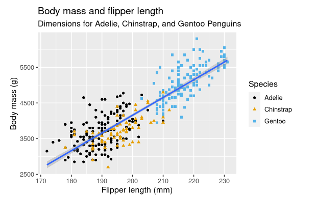
– What are the variables?
– What patterns / trend can you takeaway from this graph?
How do we make graphs?
The process
mtcars
You want to create a visualization. The first thing we need to do is set up the canvas…
The process
mtcars |>ggplot()
The process
mtcars |>ggplot(aes(x = variable.name, y = variable.name))aes: describe how variables in the data are mapped to your canvas
The process
+ “and”
When working with ggplot functions, we will add to our canvus using +
The process
mtcars |>ggplot(aes(x = variable.name, y = variable.name)) +geom_point()The process

ae-02
Recreate Graph

Wrap up: Exercises 2.3.1

Recap of AE
– Construct plots with ggplot().
– Layers of ggplots are separated by +s.
– Aesthetic attributes of a geometries (color, size, transparency, etc.) can be mapped to variables in the data or set by the user.
– Use facet_wrap() when faceting (creating small multiples) by one variable and facet_grid() when faceting by two variables.
