Modelling fish

Application exercise

For this application exercise, we will work with data on fish. The dataset we will use, called fish, is on two common fish species in fish market sales.

library(tidyverse)
library(tidymodels)

fish <- read_csv("data/fish.csv")

The data dictionary is below:

variable	description
`species`	Species name of fish
`weight`	Weight, in grams
`length_vertical`	Vertical length, in cm
`length_diagonal`	Diagonal length, in cm
`length_cross`	Cross length, in cm
`height`	Height, in cm
`width`	Diagonal width, in cm

Visualizing the model

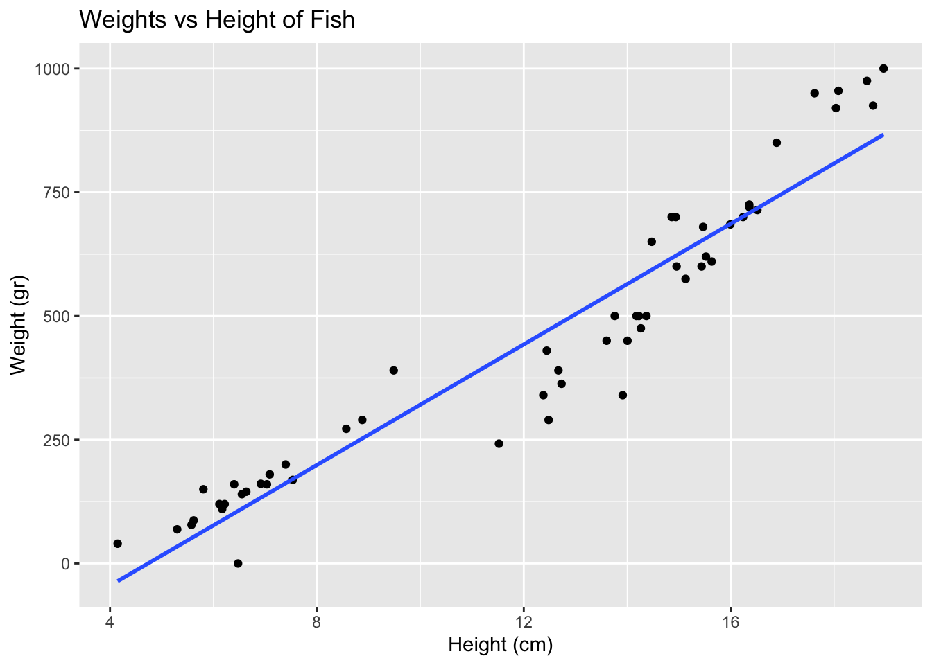
We’re going to investigate the relationship between the weights and heights of fish.

Demo: Create an appropriate plot to investigate this relationship. Add appropriate labels to the plot.

fish |>
  ggplot(
    aes(x = height , y = weight)
  ) + 
  geom_point() +
  labs(title = "Weights vs Height of Fish",
       y = "Weight (gr)",
       x = "Height (cm)")

Your turn (5 minutes):

If you were to draw a a straight line to best represent the relationship between the heights and weights of fish, where would it go? Why?

    *Add response here.*

-   Now, let R draw the line for you. Refer to the documentation at <https://ggplot2.tidyverse.org/reference/geom_smooth.html>. Specifically, refer to the `method` section.

fish |>
  ggplot(
    aes(x = height , y = weight)
  ) + 
  geom_point() +
  geom_smooth(method = "lm" , se = F) +
  labs(title = "Weights vs Height of Fish",
       y = "Weight (gr)",
       x = "Height (cm)")

`geom_smooth()` using formula = 'y ~ x'

What types of questions can this plot help answer?

Predictions and relationships between variables!

Model Prediction

Demo: Fit a model to predict fish weights from their heights.

fish_model <- linear_reg() |>
  set_engine("lm") |>
  fit(weight ~ height , data = fish)

fish_model

parsnip model object


Call:
stats::lm(formula = weight ~ height, data = data)

Coefficients:
(Intercept)       height  
    -288.42        60.92

Your turn (3 minutes): Predict what the weight of a fish would be with a height of 10 cm, 15 cm, and 20 cm using this model.

x <- c(10,15,20)

-288.42 + 60.92*x

[1] 320.78 625.38 929.98

predict(fish_model, data.frame(height = 40))

# A tibble: 1 × 1
  .pred
  <dbl>
1 2148.

Which prediction is considered extrapolation? Why?

When we predict outside the bounds of our data

Why is extrapolation important to consider when making predictions?

If we do this, we make the assumption that there is a linear relationship between x and y where we have no observed data

Model Fitting

How did R pick this line over another line? Why is this line the “best fit line”?

Residual

What is a residual?

observed value - predicted value

What do residuals look like?

Calculate predicted weights for all fish in the data and visualize the residuals under this model. Hint: We are going to use the augment function in R to get the information we need.

fish_hw_aug <- augment(fish_model$fit)

fish_hw_aug |>
ggplot(
 aes(x = height, y = weight)) + 
  geom_point() + 
  geom_smooth(method = "lm", se = FALSE, color = "lightgrey") +  
  geom_segment(aes(xend = height, yend = .fitted), color = "gray") +  
  geom_point(aes(y = .fitted), shape = "circle open") + 
  theme_minimal() +
  labs(
    title = "Weights vs. heights of fish",
    subtitle = "Residuals",
    x = "Height (cm)",
    y = "Weight (gr)"
  )

`geom_smooth()` using formula = 'y ~ x'

Model summary

Demo: Display the model summary including estimates for the slope and intercept along with measurements of uncertainty around them. Show how you can extract these values from the model output.

fish_model |>
  tidy()

# A tibble: 2 × 5
  term        estimate std.error statistic  p.value
  <chr>          <dbl>     <dbl>     <dbl>    <dbl>
1 (Intercept)   -288.      34.0      -8.49 1.83e-11
2 height          60.9      2.64     23.1  2.40e-29

Demo: Write out your model using mathematical notation.

Hint: You can type equations within dollar signs. LaTeX equations are authored using standard Pandoc markdown syntax (the editor will automatically recognize the syntax and treat the equation as math in the code chunks). It will appear as rendered math in your document.

Useful tips:

“;” is a space in Pandoc markdown (won’t use often)

More tips below:

\(x^2 \; superscript\)

\(x_2 \; subscript\)

\(\hat{x}\; adds\; hat\; to\; x\)

\(\beta \; this\; is\; beta\)

\(\epsilon\; this\; is\; epsilon\)

Our model

\(\hat{weight} = -288 + 60.9*height\)